Data Structure and Algorithm
This page cover advanced topic.
Array and Strings
| Technique | Description | Complexity |
|---|---|---|
| Two Pointer Technique | An active and passive pointer iterates | O(n) |
| Sliding Window Technique | A window slides among the array | O(n * k) → O(n) |
Given an array of integers nums and an integer target, return indices of the two numbers such that they add up to target.
# Using Hash
def twoSum(self, nums, target):
    seen = {}
    for i, v in enumerate(nums):
        remaining = target - v
        if remaining in seen:
            return [seen[remaining], i]
        seen[v] = i
    return []
Given a string s, find the length of the longest substring without duplicate characters.
# Using Set and Sliding Window
def lengthOfLongestSubstring(self, s: str) -> int:
    n = len(s)
    maxLength = 0
    charSet = set()
    left = 0

    for right in range(n):
        if s[right] not in charSet:
            charSet.add(s[right])
            maxLength = max(maxLength, right - left + 1)
        else:
            while s[right] in charSet:
                charSet.remove(s[left])
                left += 1
            charSet.add(s[right])

    return maxLength

# Using Map (Faster)
def lengthOfLongestSubstring(self, s: str) -> int:
    n = len(s)
    maxLength = 0
    charMap = {}
    left = 0

    for right in range(n):
        if s[right] not in charMap or charMap[s[right]] < left:
            charMap[s[right]] = right
            maxLength = max(maxLength, right - left + 1)
        else:
            left = charMap[s[right]] + 1
            charMap[s[right]] = right

    return maxLength
Given two sorted arrays nums1 and nums2 of size m and n respectively, return the median of the two sorted arrays.
Concepts: Binary Search & Two Pointer
Linked List
A linked list is a data structure that the node points to next node in list. Stack is FIFO, Queue is FIFO.
Given the head of a linked list, remove the nth node from the end of the list and return its head.
# Two pointers have distance of n. When the second pointer reach the end, the first pointer is the nth node from the end.
def removeNthFromEnd(self, head, n):
    """
    :type head: Optional[ListNode]
    :type n: int
    :rtype: Optional[ListNode]
    """

    count = n
    dum = ListNode()
    dum.next = head
    ptr1 = ptr2 = dum

    if not head or count == 0:
        return head

    while ptr2.next:
        if count < 1:
            ptr1 = ptr1.next
        ptr2 = ptr2.next
        count -= 1
    ptr1.next = ptr1.next.next
    return dum.next
Hash
Sometimes called as hash, hash map, map, unordered map, dictionary. A hash function maps a key to a value. It it consistent and irreversible. Suitable for quick key to value query but not the opposite.
Collision happens when two different key maps to the same value. In open addressing, the collided keys are mapped to a new index. Linear probing maps to next free index. Double hashing maps the value again with a offset. Quadratic probing maps to next offset in quadratic sequence until a free index is found. In closed addresing, a linked list is used for collided keys.
| Language | Hash | Description |
|---|---|---|
| Python | Dictionary | Use open addressing, resize at a threshold |
| C++ | Unordered Map | Use closed addressing (bucket) |
| Java | HashMap | Use bucket, change to balanced tree at a threshold |
| C | uthash library | Manual |
Tree
| Traversal | Steps |
|---|---|
| Pre-order | Root -> Left -> Right |
| In-order | Left -> Root -> Right |
| Post-order | Left -> Right -> Root |
Binary Search Tree
Binary tree index nodes in an array in BFS order. The left node of i is i*2 + 1 and right node of i: i*2 +2. Binary search tree is a binary tree where the value of the left node is less than the root node and the value of the right node is greater than the root node. This have complexity of O(log n) for search.
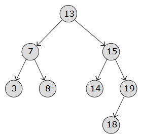
It's straight forward to insert a node. To delete a node, there's 3 condition.
- If node is leaf, delete it.
- If node has one child, replace the node with its child.
- If node has two children, find the minimum value of the right subtree (in-order traversal first successor) and replace the node with it.
Given two integer arrays preorder and inorder where preorder is the preorder traversal of a binary tree and inorder is the inorder traversal of the same tree, construct and return the binary tree.
Answer Tree:
    3
   / \
  9  20
     / \
    15  7

Input: preorder = [3,9,20,15,7], inorder = [9,3,15,20,7]

The first node in preorder is 3, which is the starting node. All the nodes before 3 in inorder are the left subtree of inorder and preorder.

The third node in preorder is 20. All the nodes before 20 in inorder are the left subtree of inorder and preorder.
# A hash mapping stores the the number as key and index as value for inorder. Construct the binary tree by preorder traversal.
def buildTree(self, preorder, inorder):
        """
        :type preorder: List[int]
        :type inorder: List[int]
        :rtype: Optional[TreeNode]
        """

        p = deque(preorder)
        h = {}
        for i in range(len(inorder)):
            h[inorder[i]] = i

        def build(s, e):
            if s > e:
                return None
            m = h[val]
            root = TreeNode(p.popleft())
            root.left = build(s, m - 1)
            root.right = build(m + 1, e)
            return root

        return build(0, len(preorder)  - 1)
Given two integer arrays preorder and inorder, construct and return the binary tree.
# The key is the current index of node in postorder must be greater than the index of parent node in preorder. Traverse the binary tree by postorder traversal.
def constructFromPrePost(self, preorder, postorder):
    """
    :type preorder: List[int]
    :type postorder: List[int]
    :rtype: Optional[TreeNode]
    """
    po = list(postorder)
    pr = {}
    for i, n in enumerate(preorder):
        pr[n] = i

    def build(i):
        parent_index = pr[i]
        if not po:
            return None
        else:
            current_node = po[-1]
        if pr[current_node] < parent_index:
            return None

        root = TreeNode(po.pop())
        root.right = build(current_node)
        root.left = build(current_node)

        return root

    return build(po[-1])
Radix Tree
Stores prefix in an efficient way.
    api/
  /      \
user/  product/
/  \    /   \
id get  id get
Heap (Priority Queue)
A min(max) heap is a tree that the children of a node is always greater(lesser) than or equal to its parent. The root is the minimum(maximum) value. This have complexity of O(log n) for insert and delete.
Initially, a binary tree looks like this. Let's make a max heap.
    10
  /    \
 20      5
/  \    / \
6    1  8   9
Heapify starts at the last non-leaf node and move upwards. In this case, start from 20. It's childern is less than 20. Move upwards, 20 is greater than 10, so swap.
        20
    /    \
    10      5
/  \    / \
6    1  8   9
Continue until a maxheap is created.
        20
    /    \
    10      5
/  \    / \
6    1  8   9
After inserting a node, heap to the root. After delete the root node, move the final leaf to the root and heap.
AVL Tree
Derived from BST. But it keeps the balance of the tree when a node is inserted by making sure difference between left and right subtree is less than 2. Balance Factor, BF = height of left subtree - height of right subtree. If BF > 0, the node is right heavy. If BF < 0, the node is left heavy.
| Case | Description | Solution |
|---|---|---|
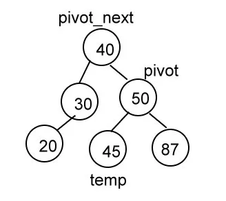
| LL | node and left child are left heavy | Rotate right |
| RR | node and right child are right heavy | Rotate left |
| LR | node is left heavy and left child is right heavy | Rotate left on left child then right on node |
| RL | node is right heavy and right child is left heavy | Rotate right on right child then left on node |
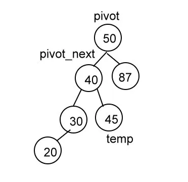
temp = pivot_next.rlink
pivot_next.rlink = pivot
pivot.llink = temp
Red-black Tree
Similar to AVL, but do lesser operation for insert and delete. AVL is better for frequent search with balanced tree.
Rules
- New node is always red
- Root is always black
- All leaves including null are black
- Nodes must be red or black
- Child of red must be black
- All path from root to leaves must has the same number of black nodes
Operations for Fixing Violation
- If parent and uncle are red, make parent and uncle black and grandparent red. Then, fix at gradparent.
- If uncle is black, node is grandparent right(left) of right(left) child, make parent black and grandparent red and rotate left(right) at gradparent. Then, fix at grandparent.
- If uncle is black, node is grandparent left(right) of right(left) child, rotate left(right) at parent (This leads to 2). Then, fix at parent.
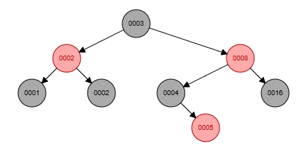
Imagine inserting on this sequence: 16, 8, 4, 2, 1, 3, 2, 5
Reference: Intro, Detail, visualization
Fenwick Tree
Efficiently compute prefix sum. For search and insert, it takes O(log n).
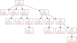
Properties
a = [1, 2, ... , n]
lsb(i) = i & -i (& denotes bitwise AND)
Parent of node i = i - lsb(i) = i & (i-1). Try to observe the bits in the image, what the lsb is doing.
At level k, there is C(log2 n, k) combination of nodes. Ex: C(3, 2) = 2^0 + 2^1, 2^0 + 2^2, 2^1 + 2^ = (3, 5, 6)
A node have lsb(i)
F[i] = sum of `(a[i - lsb(i)], a[i]]`
# Interrogation (Query)
To search a range of prefix sum, let say i, j = [7, 8]. The common ancestor must be j - lsb(j), that is 0. Subtract F[j] from F[i]. Currently, F[8] contains sum of `a(0, 8]`, F[7] contains sum of 7. Then we continue iterate so new_i = i - lsb(i), which is the parent of F[i]. Now new_i is 6, we subtract (F[8] - F[7]) from F[6]. F[6] contains sum of 5 and 6. Continue until i != j - lsb(j). We will get the prefix sum of 8 and 7. That results in a[8]
# Update
Here, the parent of a node is different: i + lsb(i) = (i|(i - 1)) + 1. Let say we update node 6 by +3. The parent of 6 is 8. Change F[6] += 3. Then, continue update i's parent recursively until i exceed n. The parent of 6 is 8. Change F[8] += 3. The parent of 8 is 16. We stop here.
When we search F[1, 5] theres no update. When we search F[6], we include the updated value. When we search F[7], it will adds the parents: F[4], F[6], F[7], the updated value is included. When we search F[14], it will adds the parents: F[8], F[12], F[14], the updated value is included.
# Search Rank
Given a prefix sum, we can calculate rank in O(log n). Nodes with odd indexes lsb(i) = 1 are leaves. Node i parent is (i - lsb(i) | 2 lsb(i)), node i child is i +- lsb(i) / 2. It looks like this:
4
/ \
2 6
/ \ / \
1 3 5 7
Let say we want to find rank of an integer F[3]. Start at root, F[3] < F[4], traverse left. F[3] > F[2], traverse right. Now we got the answer. The index of 3 is 6. From index 6, we can calculate the rank is 3.
Graph
Shortest Path
Dijkstra's Algorithm
Find shortest path from one vertex to all other vertex. Does not work for negative edge weight.
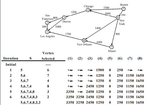
Find min{current cost from v to u, cost from current vertex to u}
Bellman-Ford Algorithm
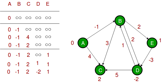
Find shortest path from one vertex to all other vertex. Work for negative edge weight. Slower than Dijkstra. If distv > distu + weight of edge uv, then update distv
Floyd-Warshall Algorithm
Finds shortest path from every vertex to all other vertex. Work for negative edge weight. Slower than Dijkstra and Bellman-Ford. In a matrix i,j, if (i, k) + (k, j) < (i, j), then update.
A* Search
At a node, approximate the distance of the next node to the goal. Then pick the shortest approximate.
Minimum Spanning Tree
A tree in a graph that only contains all of the vertex of the graph with smallest total weight
Kruskal's algorithm
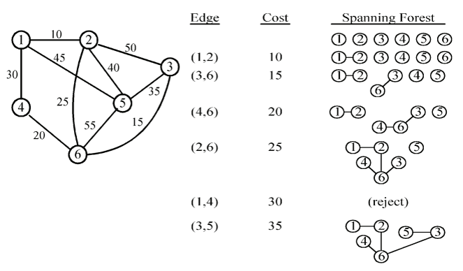
- Select edge with smallest weight
- Add the next smallest weight edge to forest if it does not cause a cycle
- Stop if there is n-1 edges, else goto step 2
Prim's Algorithm
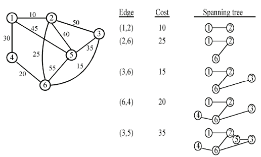
- x in V, A = {x}, B = V - {x}
- Select (u, v) where u in X, v in Y such that (u, v) has smallest weight between A and B. Memorizing the minimal discovered edge
- Put (u, v) in tree. A = A U {v}, B = B - {v}
- If B = empty, stop, else, go to step 2
Cycle Basic
Cycle basis is set of cycles that can generate every cycle in graph using ring sum operator (linear combination).
- Determine size of minimal cycle basis as k
- Find all cycles and sort by weight. Add cycles to cycle basis one by one if it cannot be formed by combination of some cycles already in cycle basis. Using Gaussian Elimination
- Stop if cycle basis has k cycles
k= |Edge Count| − (|Vertex Count| − 1)
Sort
| Method | Steps | Best | Average | Worst |
|---|---|---|---|---|
| Insertion Sort | Iterate and move smaller element to the left until correct position | O(n) | O(n^2) | O(n^2) |
| Selection Sort | Iterate and move smallest element to the first element | O(n) | O(n log n) | O(n^2) |
| Bubble Sort | Iterate and move largest element to the last element | O(n) | O(n^2) | O(n^2) |
| Method | Steps | Complexity |
|---|---|---|
| Merge Sort | Divide and sort at each merge | O(n log n) |
| Quick Sort | Partition and sort recursively | O(n^2) |
| Heap Sort | Refer to heap | O(n log n) |
| Knowckout Sort | Tournament rule the largest at the root and the next largest at the child of the parent | O(n log n) |
| Huffman Algorithm | A tree is constructed by joining two subtree or leaves with the least frequency | O(n log n) |
| Counting Sort | Count the number of each element and sort | O(n + k) |
| Radix Sort | Sort based on each digit | O(n * k) |
| Bucket Sort | Hash on n buckets each with a linked list using insertion sort | O(n) |
def quicksort(arr):
    if len(arr) <= 1:
        return arr
    else:
        pivot = arr[0]
        # all element lesser than pivot is put into this array
        less = [x for x in arr[1:] if x <= pivot]
        # all element greater than pivot is put into this array
        greater = [x for x in arr[1:] if x > pivot]
        return quicksort(less) + [pivot] + quicksort(greater)
unsorted_array = [3, 6, 8, 10, 1, 2, 1]
sorted_array = quicksort(unsorted_array)
print("Unsorted array:", unsorted_array)
print("Sorted array:", sorted_array)
Recursive
Divide and Conquer
Divide problem into subproblem resursively.
2D-Rank Finding O(n log n)
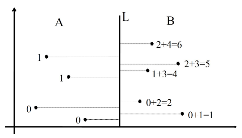
- Sort all points based on x then y
- Find median line
- Find ranks of points in A and B recursively
- Update ranks of points B when the y value of points in B is greater than A
Closest Pair Problem O(n log n)
Find the closest point in a graph of points. Source.
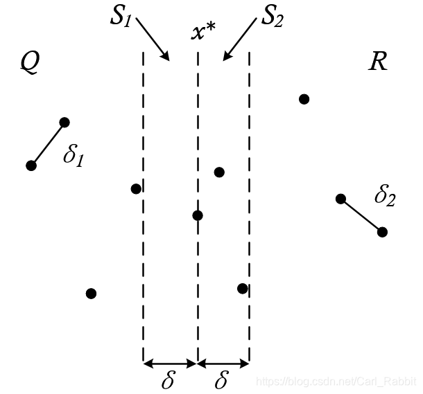
- Pick a median x point and divide into 2 part recursively. Use brutal when points <= 3
- On merging, find the min pairs from SL(left region), SR(right region), or closest pair that lies in (median + d, median - d). d is the min pair distance in SL and SR. Let p be a point in SL, the y of q in SR side of slab must be in between p.y + d, p.y - d
Convex Hull - Graham's Scan (Greedy)
Find smallest convex polygon containing all of the points.
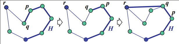
- Find lowest point. O(n)
- Form nonintersecting polygon by sorting the points counterclockwise. O(n log n)
- Remove nonconvex vertex. O(n)
Voronoi Diagram
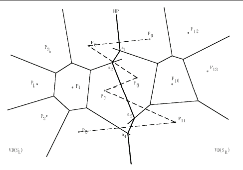
Branch and Bound
Personnel Assignment Problem
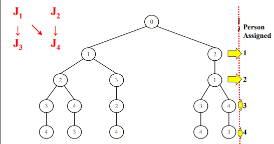
Each personal work each jobs at different cost. Some jobs need to be done before other jobs. Use topological sort to display as branch.
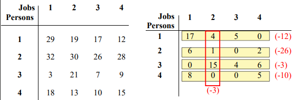
Calculate reduced cost matrix. So that in every branch and bound, we can determine which branch have minimum lower bound.
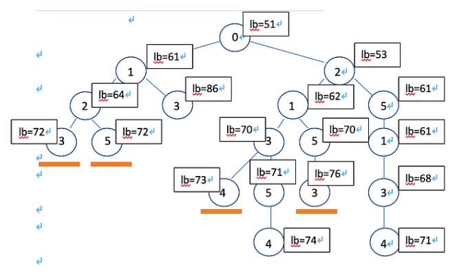
The final flow is 0, 2, 5, 1, 3, 4 because at each branch, the node have lower bound.
Learn further about this concept on travelling salesman problem.
Knapsack Problem (Branch and Bound)
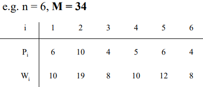
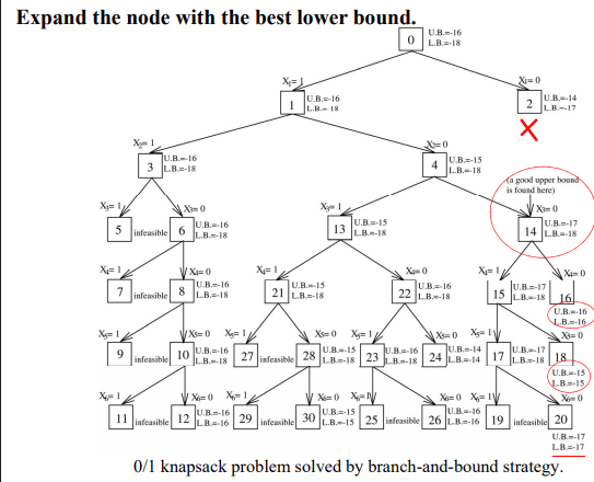
The upper bound found by a feasible solution. (Picks the most points first). The lower bound is found greedy. (Calculate the density and get allowing weights to be fractured, P1 + P2 + 5/8 P3).
Linear Programming (Prune and Search)
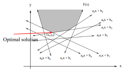
Slice things.
Dynamic Programming
Use memory to save computated values for future use.
Longest Common Subsequence
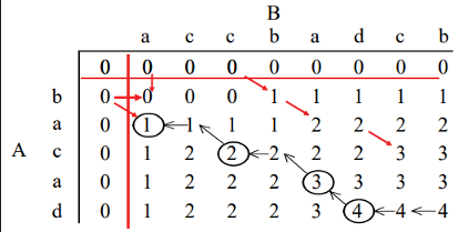
A = "bacad", eg: ad, ac, bac, acad, bacad, bcd
B = "accbadcb", eg: ad, ac, bac, acad
LCS of A and B: acad
Knapsack
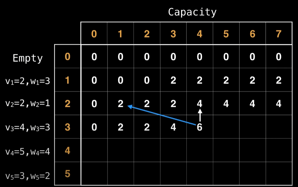
i is the total weight, j is the turn of items. In each turn, the vertical arrow suggest now taking that item, the diagonal shift suggest taking that item by shifting n units to the left by the weight. The cell indicates the maximum value of not taking the item (vertical) or take the item max value at reduced weight + current value (diagonal).
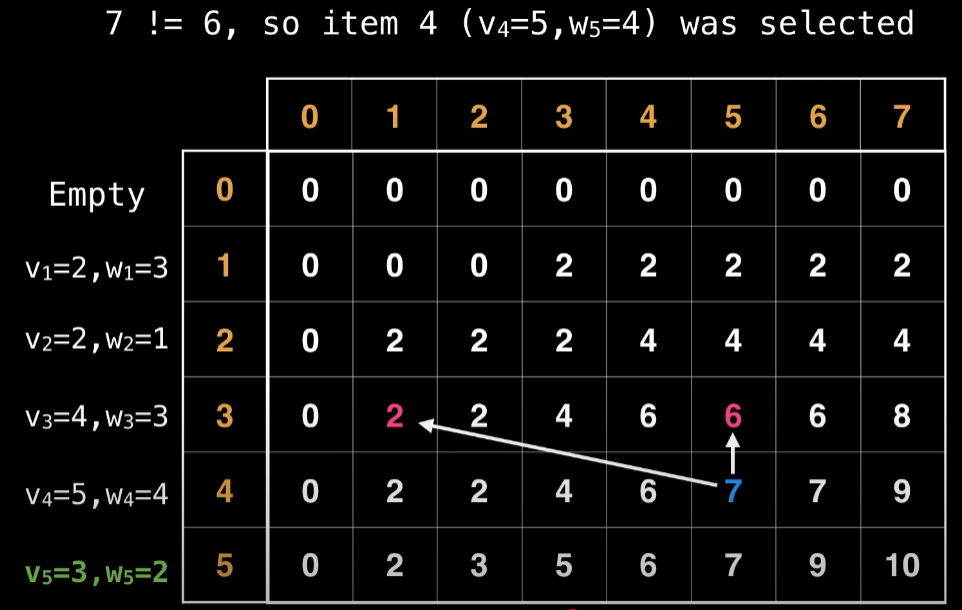
To find the optimal results, if the vertical arrow shows same number as the cell. Don't take that item.
Given an integer array nums, find a subarray that has the largest product, and return the product.
def maxProduct(self, nums):
    """
    :type nums: List[int]
    :rtype: int
    """
    res = max(nums)
    cur_max = cur_min = 1
    for n in nums:
        ma = cur_max * n
        mi = cur_min * n
        cur_max = max(ma, mi, n)
        cur_min = min(ma, mi, n)
        res = max(res, cur_max)

    return res
Given an integer array nums, return the length of the longest strictly increasing subsequence.
Example 1:
Input: nums = 10,9,2,5,3,7,101,18 Output: 4
# Replacing an element (Let's sat 3 replace 5, because both are greater than 2) in the result lis did not increae the number of LIS.
def lengthOfLIS(self, nums):
        """
        :type nums: List[int]
        :rtype: int
        """
        def binarySearch(key, li):
            left = 0
            right = len(li) - 1
            while left <= right:
                m = (left + right) // 2
                if key > li[m]:
                    left = m + 1
                elif key < li[m]:
                    right = m - 1
                else:
                    return m
            return left

        lis = list()

        for i in range(len(nums)):
            n = nums[i]
            if not lis or lis[-1] < n:
                lis.append(n)
            else:
                inx = binarySearch(n, lis)
                lis[inx] = n

        return len(lis)
Backtracking
Backtracking is a problem-solving algorithmic technique that involves finding a solution incrementally by trying different options and undoing them if they lead to a dead end.
Advanced Data Structure
Randomized Algorithm
Use randomess to solve problems.
| Feature | Las Vegas Algo | Monte Carlo Algo | Deterministic Algo (Normal) |
|---|---|---|---|
| Correctness | Always | High probability of correctness | Always |
| Time by same input | Varies | Constant & controlled | Constant |
| Examples | Randomized Quicksort | 1/2 Approximate Median | Quicksort |
Rabin-Karp Algorithm
A string-searching algorithm that uses hashing.
text = ABCDEFCDE
pattern = CDE
result = [2, 6] (index of substring is same as pattern)

# Steps

Let a = 1, b = 2, ...
Hash(CDE) = (a * 100 + b * 10 + c) mod 13 = 7 = Hash(pattern)
Hash(ABC) = (1 * 100 + 2 * 10 + 3) mod 13 = 6
Hash(BCD) = (2 * 100 + 3 * 10 + 4) mod 13 = 0   # This can be optimized to improve from O(mn) to O(m + n) as below
Hash(BCD) = ( (Hash(BDC) - a * 100) * 10 + d ) mod 13 = 0
Hash(BCD) = ( (0 - 1 * 100) * 10 + 4 ) mod 13 = 0

If Hash(pattern) = Hash(CDE), check manually if the substring is same.
Knuth-Morris-Pratt Algorithm
This algorithm is efficient for finding number of occurence of a pattern in a string in O(n). It creates an auxiliary array (LPS) for the pattern that store the previous starting point. Then, we iterate through the string and check if the pattern matches.
def lps(pattern):
    m = len(pattern)
    lps = [0] * m
    i, j = 1, 0
    while i < m:
        if pattern[i] == pattern[j]:
            j += 1
            lps[i] = j + 1
            i += 1
        else:
            if j == 0:
                lps[i] = 0
                i += 1
            else:
                j = lps[j - 1]
    return lps

def kmp(text, pattern):
    n = len(text)
    m = len(pattern)
    lps = lps(pattern)
    i = j = 0
    while i < n:
        if text[i] == pattern[j]:
            i += 1
            j += 1
        if j == m:
            print("Found at: ", i - j)
            j = lps[j - 1]
        else:
            if i < n and text[i] != pattern[j]:
                if j == 0:
                    i += 1
                else:
                    j = lps[j - 1]
            else:
                i += 1
Segment Tree
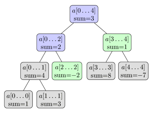
Stores range values. The picture shows finding sum of interval 2, 4 by adding a2...2 and a3...4. To update a value, iterate the update using divide and conquer.
Future Studies
DSA
- Topological Sorting
- Max Flow / Min Cut (Ford-Fulkerson, Edmonds-Karp, Dinic): For graph-based resource allocation, network flow, image segmentation
- Strongly Connected Components (Tarjan / Kosaraju)
- Union-Find (Disjoint Set Union)
- Graph Coloring / Bipartite Checking
- Bitmask DP: Compress states, used for NP-hard approximation like Traveling Salesman Problem (TSP)
- Digit DP / Interval DP / Memory-efficient DP
- Trie + Bit Trie: String search, XOR maximization
- Suffix Array / Suffix Tree / LCP: String processing, genome comparison, compression
- Persistent Data Structures: Time travel, version control
- Convex Optimization / Lagrange Multiplier
- Online Algorithms / Competitive Analysis
- Parallel / Distributed Algorithms
Numerical Computing
- Linear Programming / Simplex
- Greedy correctness with Matroids
- Combinatorics, Generating Functions